Introduction to ANOVABNPTestR

library(ggplot2)
library(ANOVABNPTestR) 
# Remember: you must call ANOVABNPTestR::setup() at least one time

To explore the basic capabilities of ANOVABNPTestR, we’ll use the simulated dataset example_01. This dataset contains 1.000 registers, a continuous response (y) and 2 factors (x1 and x2), with x1 == x2 == 1 representing the control group.

First, let us plot a boxplot of y for each combination of x1 and x2:

data <- ANOVABNPTestR::example_01
data |>
  ggplot2::ggplot(ggplot2::aes(y = y)) + 
  ggplot2::geom_boxplot() +
  ggplot2::facet_wrap(
    nrow = 1,
    ggplot2::vars(x1, x2), 
    labeller = "label_both"
  ) +
  ggplot2::theme_classic(base_size = 15) + 
  ggplot2::theme(
    panel.spacing = ggplot2::unit(1, "lines"),
    axis.title.x = ggplot2::element_blank(),
    axis.ticks.x = ggplot2::element_blank(),
    axis.text.x = ggplot2::element_blank()
  )

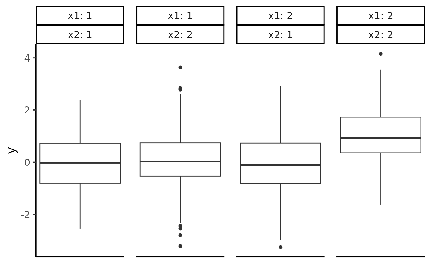
This plot suggests that the only different cell is the one with x1 == x2 == 2. However, without a formal test, we cannot be sure. ANOVABNPTestR solves this issue using a BNP model.

Fitting the model

First, we must fit the model. As our responses take values on the real line, we can use anova_bnp_normal() (see anova_bnp_berpoi() for counts and anova_bnp_bernoulli() for Boolean variables):

yvec <- example_01[[c("y")]]
Xmat <- example_01[, c("x1", "x2")] |> as.matrix()
my_fit <- ANOVABNPTestR::anova_bnp_normal(yvec, Xmat)